Highlight Key Metrics with Excel Conditional Formatting.

Visual cues help us grasp situations at a glance. When driving, for example, colored lights tell us whether to stop, go or pull over so emergency vehicles can pass. We could never read highway conditions as quickly without them.

The same is true with large data sets. That’s why Excel’s conditional formatting is so useful — it lets us set up easy-to-read signals that highlight our data.

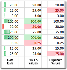
How Does Conditional Formatting Work? Conditional formatting changes cell appearance based on rules we assign. For example, it can highlight the highest and lowest values in a list or flag duplicate entries. Best of all, the formatting updates automatically as the data change.

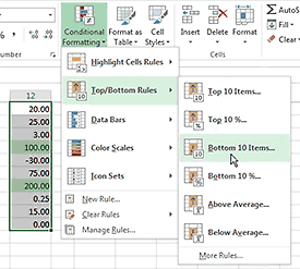
How Can I Set Up Conditional Formats? Everything is under the Conditional Formatting button on the Home ribbon.¹ The following example shows how to apply conditional formatting that highlights the two highest and two lowest values in a list:

1. Select the cells to be formatted;
2. Press the triangle on the Conditional Formatting button to display the menu (See Figure 1);
3. Choose Top/Bottom Rules and then Top 10 Items;
4. When the dialogue box opens, change the number 10 to 2 and pick the Green format;
5. Repeat steps 3 and 4, but this time pick Bottom 10 Items and choose the Red format.

Now the cells with the two highest values will be green and those with the two lowest will be red.

What Happens When Two or More Formats Apply to the Same Cell? Our high/low example shows two rules being applied to the same data: one for high values and another for lows. But the high and low formats will never both apply to the same cell as long as there are at least four different values in the list.

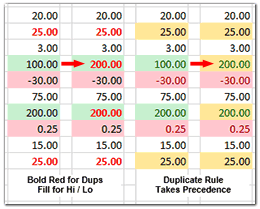
But suppose we want to highlight both duplicates and high/low values. Both rules will apply to any cell that is both a high or low value and also a duplicate. Since Excel’s default formats for highs/lows and duplicates both use fill and font color, we need to indicate which color to use when both conditions apply.

Figure 2 shows two solutions. The red arrows point to a cell whose value changes from 100 to 200. The number 100 was already a top two value in the list, but when it increases to 200 it also becomes a duplicate. The solution on the left uses fill color to mark high/low values and font color for duplicates. When 100 changes to 200, the font turns red to indicate a duplicate while the fill remains green since 200 is a top value.

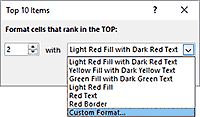
To specify these formats, pick Custom Format when defining the rules. Then choose the desired font and fill colors from the Format Cell dialogue box (See Fig. 3).

The solution on the right is to give one of the formats precedence in a conflict. In our case, yellow shows duplicates, green top values and red bottom values. The duplicates rule is given priority so that when the value 100 changes to 200, the fill becomes yellow since the duplicates rule was given precedence.

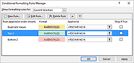
Rule priority is specified in the Conditional Formatting Rules Manager (See Figure 4). To make this setting, you first have to create the rules and apply them to the cells to be formatted. Then, select the cells to be formatted and choose Manage Rules from the bottom of the Conditional Formatting menu. All rules assigned to the selected cells are listed; those on top take precedence over those below. You can rearrange the list to create the desired hierarchy.

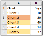
Can a Cell’s Format Be Conditioned on Values in Other Cells? Sometimes we may want to format one cell based on values in others. For example, an accounts receivable person may want a client’s name to be yellow if an invoice has been outstanding more than 30 days and red after 45 (See Figure 5).

This requires two rules: one for values greater than 30; another for those over 45. The following steps create the over 30 rule:

1. Select the cells to be formatted (A2 to A6 in the example);
2. Choose New Rule from the Conditional Formatting menu;
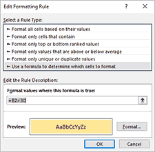
3. Pick “Use a formula …” as the rule type (See Figure 6);
4. Click in the formula box;
5. Enter the formula “=B2>30” (B2 is the cell containing the first entry for Days);
6. Click the Format button and specify the desired appearance; and
7. Click OK.

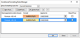
Repeat the same steps to create a rule for over 45 days. The formula should be “=B2>45”. Then open the Manage Rules dialogue box and make sure the 45 day rule is on top (See Figure 7).

This example may not seem very useful since we could easily apply these formats to the number of days in column B using Excel’s built-in conditional formats. In the real world, however, the account aging data could be in a remote area or even on a different sheet. In fact, we could build a conditional format formula that computed the days outstanding from the invoice date and TODAY function and tested whether that amount was greater than 30 or 45.

Absolute or Relative Cell Reference? In the account aging example, the formula B2>30 is the test for cell A2. For cell A3, however, the test should look at the number in B3, for A4 to the number in B4 and so on down the list. Excel will make these adjustments automatically if we enter the equation for the first cell in the list (A2 in the example).

Sometimes, however, we don’t want the referenced cell to be adjusted like that. For example we want to compare every entry in a list to a goal specified in B2. To “lock” a cell reference so it won’t be adjusted, put dollar signs in it, for example $B$2.² This is called an absolute cell reference; entries without dollar signs are called relative cell references.

* * * * *

The old adage that one picture is worth a thousand words has never been truer than today. Our ability to gather data has grown exponentially while our ability to analyze it has not. Scientists and business people are trying to close the gap by summarizing and highlighting key information with data visualization tools. Excel’s conditional formatting provides a convenient and powerful vehicle for doing this.

-----

1. Applies to Excel 2007 and newer. In Excel 97 to 2003 conditional formatting is on the Format menu.
2. The entry $B$2 locks both the row and column references. $B2 locks only the column and B$2 only the row.

Conditional formatting is covered in our Excel Dashboards class.

Visit our Excel Productivity Guides page for more helpful articles.

This article originally appeared in our free twice-monthly e-mail newsletter. To receive future issues, please add your name to the subscription list.

Want to learn more? We offer seven different Excel classes: Mastering Excel, Advanced Excel, Excel Charts, Excel Dashboards, Macros and Pivot Tables and Power Pivot. Click any class name for a detailed description.

We can also create a private Personalized Excel Class for your group, or provide individual training or project consulting services.