Seven Excel Tips for 2019.

Everyone likes to get a fresh start for the New Year. Here are a few simple things you can do in Excel that will make you more productive.

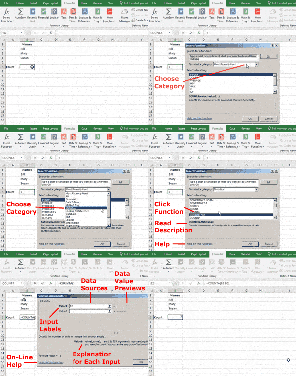
Use the Insert Function Button. When you use functions in an equation, enter them with the Insert Function button (fx) rather than by typing. Here are the benefits (see Fig. 1.):

1. The button opens a dialogue box that lists all functions by category. This lets you explore and learn about useful functions you might not be familiar with. Clicking any function’s name displays a brief description.
2. When you choose a function and click OK, a second dialogue box opens telling you what information the function needs and where to put it. As you enter this information, an explanation of each entry appears at the bottom. A link at the bottom left brings up the help page for that function on the Microsoft web site.
3. As information is entered, the input values and computed result are previewed. This helps catch errors while the equation is being set up.

Obviously, it’s sometimes faster to type simple functions you use every day. But even experienced users find this often overlooked feature helpful for new and infrequently used functions.

Click to Insert Cell References. Typos in formulas are fatal. If you type “M10” instead of “N10,” Excel won’t know it’s a mistake and will compute the wrong result.

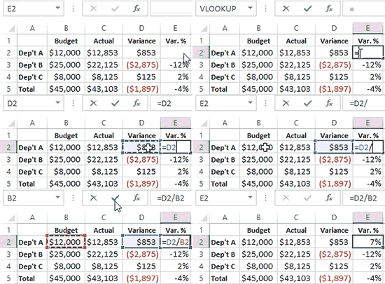
An easy solution is to enter cell references with the mouse. Simply type an equal sign and then click on the cell(s) you want to reference (see Fig. 2). This method is particularly useful when a referenced cell is on an another worksheet or workbook since the click enters not only the cell, but also the appropriate reference to its sheet or workbook.

As a formula is built, Excel outlines the referenced cells with colored boxes. This makes it easy to spot errors where the formula refers to the wrong cells, although it won’t catch errors like typing a plus sign when minus was intended.

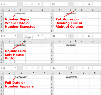
Number Signs Appear Where a Date or Number is Expected. This is not an error, but simply an indication that the column isn’t wide enough. Adjust the column width and the date or number should display correctly (see Fig. 3). Double clicking the divider between the column headings will automatically resize the column to accommodate the largest entry.

Formulas that Refer to Data in Other Workbooks. When creating a formula that references data in another workbook, be sure both the workbook containing the formula and the one with the data are saved in the places and with the names where you intend to keep them. The formula includes both the workbook’s name and location, so if either changes, all formulas referencing the workbook will need to be updated.

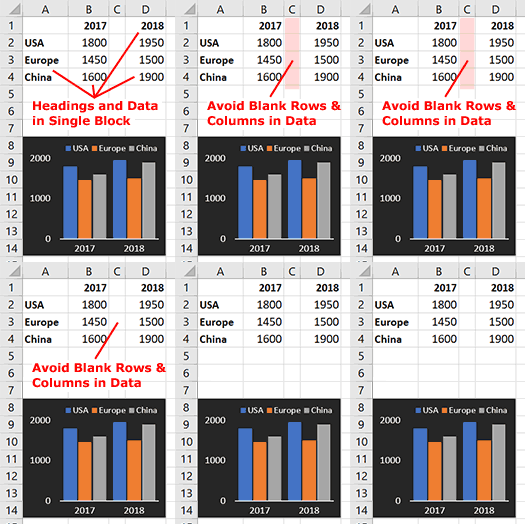
Set Up Data for Charts. If you want to create a chart, it’s usually easiest to organize the source data as follows (see Fig. 4):

1. Arrange all the data and headings in one block.
2. Don’t put blank rows or columns within the data zone.
3. If the first row or left-most column contains labels, not data, keep the top or left-most cell blank to help Excel figure out which entries are headings.

Keyboard Shortcut. To select a rectangular block of data, click on any non-blank cell within the data area. Then hold the control (command key on Mac) while typing “A.” Excel will extend the selection outward in all four directions until it reaches clear rows and columns.

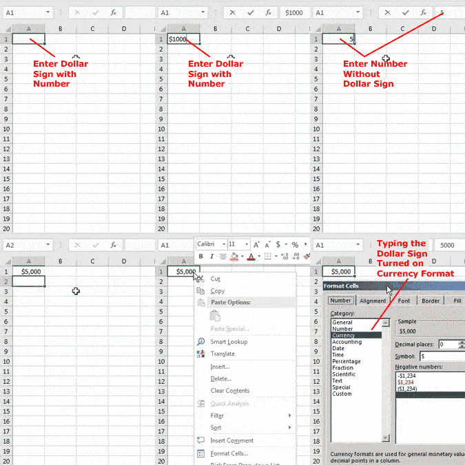
Formatting Belongs to a Cell, Not Its Content. If you’ve ever found yourself unsuccessfully trying to delete a dollar or percent sign that doesn’t seem to be there, here is the reason: Those symbols are part of a number format even if you initially typed them. Here’s how it works (see Fig. 5.).

When you type a number with a dollar or percent sign, Excel never actually enters the dollar or percent character in the cell, rather uses the keystroke as a trigger to turn on currency or percent formatting. Thus, there is no dollar or percent sign character to delete.

Even if you delete everything in the cell and start fresh, the dollar or percent sign will return. This is because cell formats such as font, border and number format are properties of the cell, not its content. Thus, to remove the dollar or percent sign you need to change the number format. If you want start formatting from scratch, select the cell and choose Clear Format from the Home Ribbon. This resets all cell formats to the document’s default.

* * * * *

Sometimes little things get overlooked, but they can make a big difference. If these tips save you ten minutes a day, that adds up to a full work week per year. That’s the power of training:

Scientia potentia est …
knowledge is power.

These tips are covered in our Mastering Excel and Advanced Excel classes.

Visit our Excel Productivity Guides page for more helpful articles.

This article originally appeared in our free twice-monthly e-mail newsletter. To receive future issues, please add your name to the subscription list.

Want to learn more? We offer seven different Excel classes: Mastering Excel, Advanced Excel, Excel Charts, Excel Dashboards, Macros and Pivot Tables and Power Pivot. Click any class name for a detailed description.

We can also create a private Personalized Excel Class for your group, or provide individual training or project consulting services.